Файл:Jordan illustration.png
Памер папярэдняга прагляду: 634 × 599 пікселяў. Іншыя разрозненні: 254 × 240 пікселяў | 508 × 480 пікселяў | 812 × 768 пікселяў | 1 064 × 1 006 пікселяў.
Арыгінальны файл (1 064 × 1 006 кропак, аб’ём файла: 55 KB, тып MIME: image/png)
| Апісанне |
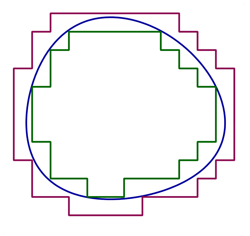
English: A set (represented in the picture by the region inside the blue curve) is Jordan measurable if and only if it can be well-approximated both from the inside and outside by simple sets (their boundaries are shown in dark green and dark pink respectively). |
| Дата | |
| Крыніца | Уласная праца |
| Аўтар | User:Oleg Alexandrov |
Тлумачэнне
Made by myself with Matlab.
| Я, уладальнік аўтарскіх правоў на гэты твор, перадаю яго ў грамадскі набытак. Дазвол сапраўдны для ўсяго свету. У некаторых краінах гэта не можа быць юрыдычна магчыма; калі так, то: Я дазваляю кожнаму выкарыстоўваць гэтую працу ў любых мэтах, без аніякіх умоваў, калі толькі такія ўмовы не патрабуюцца паводле закону. |
Ліцэнзіяванне
| Я, уладальнік аўтарскіх правоў на гэты твор, перадаю яго ў грамадскі набытак. Дазвол сапраўдны для ўсяго свету. У некаторых краінах гэта не можа быць юрыдычна магчыма; калі так, то: Я дазваляю кожнаму выкарыстоўваць гэтую працу ў любых мэтах, без аніякіх умоваў, калі толькі такія ўмовы не патрабуюцца паводле закону. |
Source code (MATLAB)
function main()

   % the function whose zero level set and inner and outer approximations will be drawn
   f = inline('60-real(z).^2-1.2*imag(z).^2-0.006*(real(z)-6).^4-0.01*(imag(z)-5).^4', 'z');

   M=10; i=sqrt(-1); lw=2.5;
   figure(1); clf; hold on; axis equal; axis off;

   if  1==0
      for p=-M:M
	 for q=-M:M
	    z=p+i*q;
	    if f(z)>0
	       plot(real(z), imag(z), 'r.')
	    else
	       plot(real(z), imag(z), 'b.')
	    end
	 end
      end
   end

% draw the zero level set of f
   h=0.1;
   XX = -M:h:M; YY = -M:h:M;
   [X, Y] = meshgrid (XX, YY); Z = f(X+i*Y);
   [C, H] = contour(X, Y, Z, [0, 0]);
   set(H, 'linewidth', lw, 'EdgeColor', [0;0;156]/256);

% plot the outer polygonal curve
   Start=5+6*i; Dir=-i; Sign=-1;
   plot_poly (Start, Dir, Sign, f, lw, [139;10;80]/256);

% plot the inner polygonal curve
   Sign=1; Start=4+5*i;
   plot_poly (Start, Dir, Sign, f, lw, [0;100;0]/256);

%  a dummy plot to avoid a matlab bug causing some lines to appear too thin
   plot(8.5, 7.5, '*', 'color', 0.99*[1, 1, 1]);
   plot(-4.5, -5, '*', 'color', 0.99*[1, 1, 1]);

   saveas(gcf, 'jordan_illustration.eps', 'psc2');

function plot_poly (Start, Dir, Sign, f, lw, color)

   Current_point = Start;
   Current_dir   = Dir;

   Ball_rad = 0.03;

   for k=1:100

      Next_dir=-Current_dir;

      % from the current point, search to the left, down, and right and see where to go next
      for l=1:3
	 Next_dir = Next_dir*(Sign*i);

	 if Sign*f(Current_point+Next_dir)>=0 & Sign*f(Current_point+(Sign*i)*Next_dir) < 0
	    break;
	 end
      end

      Next_point = Current_point+Next_dir;

      plot([real(Current_point), real(Next_point)], [imag(Current_point), imag(Next_point)], 'linewidth', lw, 'color', color);

      round_ball(Current_point, Ball_rad, color'); % just for beauty, to round off some rough corners

      Current_dir=Next_dir;
      Current_point = Next_point;

   end


function round_ball(z, r, color)
   x=real(z); y=imag(z);
   Theta = 0:0.1:2*pi;
   X = r*cos(Theta)+x;
   Y = r*sin(Theta)+y;
   Handle = fill(X, Y, color);
   set(Handle, 'EdgeColor', color);

|
This math image could be re-created using vector graphics as an SVG file. This has several advantages; see Commons:Media for cleanup for more information. If an SVG form of this image is available, please upload it and afterwards replace this template with
{{vector version available|new image name}}.
It is recommended to name the SVG file “Jordan illustration.svg”—then the template Vector version available (or Vva) does not need the new image name parameter. |
Гісторыя файла
Націснуць на даце з часам, каб паказаць файл, якім ён тады быў.
| Дата і час | Драбніца | Памеры | Удзельнік | Тлумачэнне | |
|---|---|---|---|---|---|
| актуальн. | 20:27, 4 лютага 2007 | | 1 064 × 1 006 (55 KB) | Oleg Alexandrov | Made by myself with Matlab. {{PD}} |
| 20:24, 4 лютага 2007 |  | 1 064 × 1 006 (55 KB) | Oleg Alexandrov | Made by myself with Matlab. {{PD}} |
Выкарыстанне файла
Наступная 1 старонка выкарыстоўвае гэты файл:
Глабальнае выкарыстанне файла
Гэты файл выкарыстоўваецца ў наступных вікі:
- Выкарыстанне ў ar.wikipedia.org
- Выкарыстанне ў ba.wikipedia.org
- Выкарыстанне ў be-tarask.wikipedia.org
- Выкарыстанне ў cv.wikipedia.org
- Выкарыстанне ў de.wikipedia.org
- Выкарыстанне ў en.wikipedia.org
- Выкарыстанне ў fr.wikipedia.org
- Выкарыстанне ў hr.wikibooks.org
- Выкарыстанне ў it.wikipedia.org
- Выкарыстанне ў ja.wikipedia.org
- Выкарыстанне ў kk.wikipedia.org
- Выкарыстанне ў ko.wikipedia.org
- Выкарыстанне ў nl.wikipedia.org
- Выкарыстанне ў pl.wikipedia.org
- Выкарыстанне ў ru.wikipedia.org
- Выкарыстанне ў uk.wikipedia.org